Angle from One Vector to Another, the Visual Way

I think most who have taken some form of higher mathematics or another will know what I mean when I say “the angle between two vectors”. I mean this:

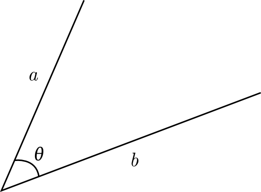
We’ve got vectors \(a\) and \(b\), and we want to get \(\theta\). But it’s pretty easy to get there - after all, we know that one definition of the dot product of two vectors is:

Solving for theta, we get a nice formula:

But, there’s a problem with this formula - the region of arccos() is all positive. If we actually want to find the angle from one vector to another, and not the angle between the two vectors, then this formula is insufficient. Imagine that \(a\) were below \(b\), and we wanted to find the angle from \(b\) to \(a\); the angle would be negative.

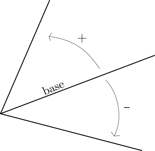
The sign of this angle doesn’t matter for most problems, but some algorithms do depend on calculating the sign. One example of an algorithm in which this matters is the funnel algorithm. Funnily enough, that algorithm is what I’m currently implementing.

In any case, for signed angles, we need a different approach. Let’s think about what I said just a bit ago - we want one vector to be the base. In the age-old case, where someone simply wants to find the angle a single vector makes with the origin, programmers learn early on that atan2f is the tool to use. Simply feed it the y and x coordinates of your vector, and it gives you back an angle. In that case, the x-axis itself is the base. It would be perfect if we could somehow make vector \(b\), in the first picture, like the x-axis.

To make sense of this, we’ll need to take a bit of a detour. The dot product is related to the angle, somehow. After all, it’s got a \(\theta\) term in it:

It’s stuck in that cosine function, though, what’s up with that? One might remember from high-school trigonometry that the cosine function has something to do with right angles. What if we just… made a right angle out of \(a\) and \(b\)?

It’s apparent that \(\cos(\theta) = \frac{\|b_0\|}{\|a\|}\), by the definition of cosine. If we substitute this definition of \(\cos(\theta)\) into the definition of the dot product above, we get:

Interesting - we now have a way to obtain \(b_0\), the segment of \(b\). This, by the way, is the scalar projection of \(a\) onto \(b\), but that’s beside the point - what does it do for us? Bear with me, we slowly approach the revelation.

Here’s where you really need to re-orient your perspective. What if \(b\) were the x-axis? No, not along the x-axis - imagine that \(b\) is the x-axis. Just humor me here. What, then, would be the y-axis? Well, maybe it’d look something like \(p\) (for perpendicular) in this picture:

We can get this perpendicular vector by rotating \(b\) 90 degrees. After simplifying the sines and cosines, this boils down to just being:

What good’s that to us? Well, let me re-orient the picture above and change up some labels:

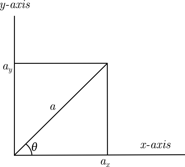
Guess what - we’ve just simplified the problem to the basic one-vector case. The angle, \(\theta\), is, of course, the same as it was before the rotation, so finding it here is equivalent. a.x and a.y are nothing but \(\|b_0\|\) and \(\|p_0\|\), respectively. Since this is essentially the one-vector case, we can just run atan2f(a.y, a.x) and we’ve got our \(\theta\).

After all this, we can finally write out our final code for obtaining the angle:

//b is considered the base
float angleBetween(Vec2f a, Vec2f b) {
    Vec2f p(-b.y, b.x);
    float b_coord = dot(a, b);
    float p_coord = dot(a, p);
    return atan2f(p_coord, b_coord);
}

If you try this with vector \(a\) below \(b\), you will see that it does indeed return a negative angle.

Note that one optimization was made in the code above: when calculating b_coord (or \(b_0\)), we don’t divide by \(\|b\|\) as we do in the formula for obtaining \(b_0\) above. Intuitively, this is because scaling a vector doesn’t change the angle it forms with another vector - \(2a\) forms the same \(\theta\) with the x-axis as \(a\). Combine that with the fact that the dot product of \(a\) and \(p\) is equal to the determinant of \(a\) and \(b\), and we can distill the algorithm into a very simple mathematical formula:

Who said trigonometry was useless? (…well, me, back in high school. But I’m trying to make a point here.)

Inkscape and WP-LaTeX used for the pictures and the math formulas, respectively.